Cathodic Protection Training Course

Cathodic Protection in relation to coatings.

The original pipeline coatings were known as 'denso tapes' though this might now be a proprietory brand name it was just a generic term in the old days.

These tapes were cloth saturated with a greasy, waxy substance and were mastic... that means they could be moulded by hand at normal temperatures. If it got too hot the grease would run out and leave a dry cloth that did not prevent corrosion.

These tapes prevented corrosion by separating the chemicals in the ground from the metal they were protecting but they were electrically conductive. (I have tested the modern Denso Mastic and it is non conductive and can therefore be used to advantage with cathodic protection.)

Cathodic protection current takes the shortest ELECTRICAL path to complete it's circuit and conductive tape allows current a short route to the negative connection of the cathodic protection system.
It is found that cathodic protection influence will not spread where conductive coatings are used and that the corrosion prevention is limited to the immediate area of influence of a groundbed or sacrificial anode.



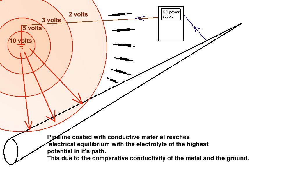
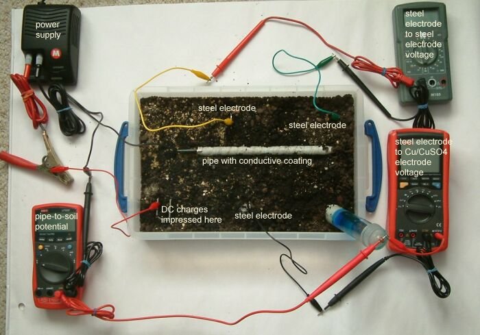
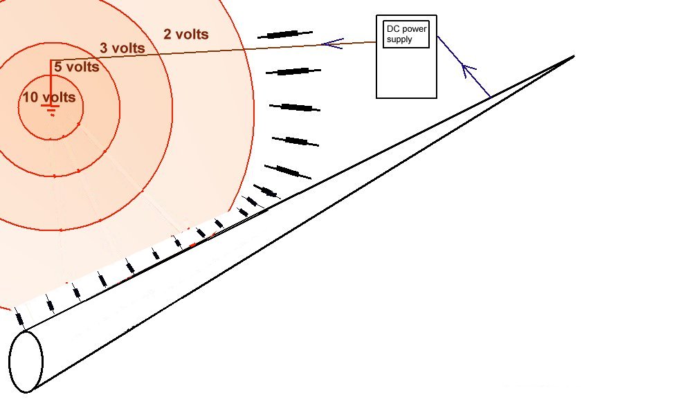
This picture shows the point at which the charges are impressed into the ground and how they raise the potential as they difuse through 'shells of resistance' towards 'remote earth'.

It shows that the potential gradiant overlaps the path of the metal of the pipeline that is connected to the negative terminal of the transformer rectifier, or DC power supply.

The picture shows that charges that are travelling towards remote earth meet a shell of resistances greater than the meet when passing direct onto the pipeline that has conductive coating.
Kirchoff defined the behaviour of charges under these conditions and we can use his laws to calculate that the charges will not spread further along the pipeline.
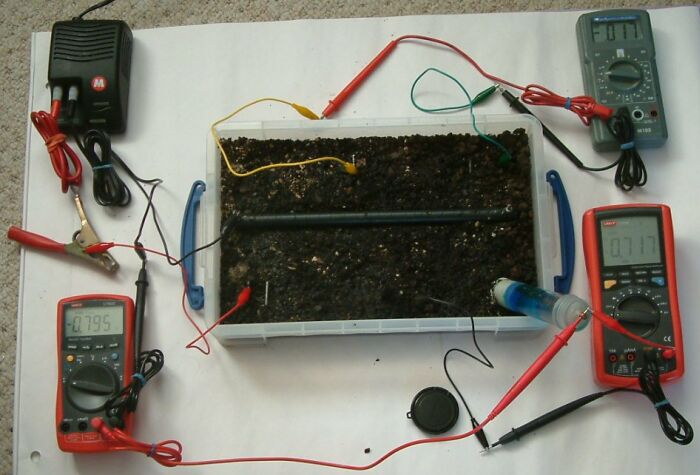
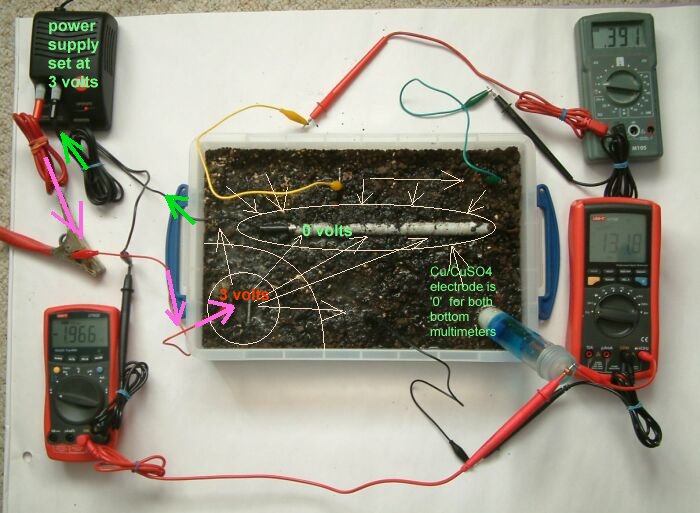
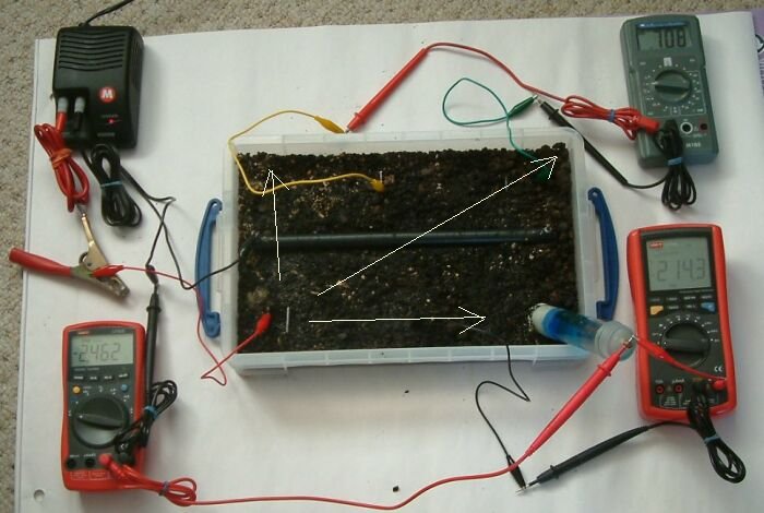
This can be demonstrated using a plastic tray full of wet earth, a short length of pipe wrapped in conductive material, a DC power supply 3 voltmeters 3 ground contact electrodes and a Cu/CuSO4 electrode.



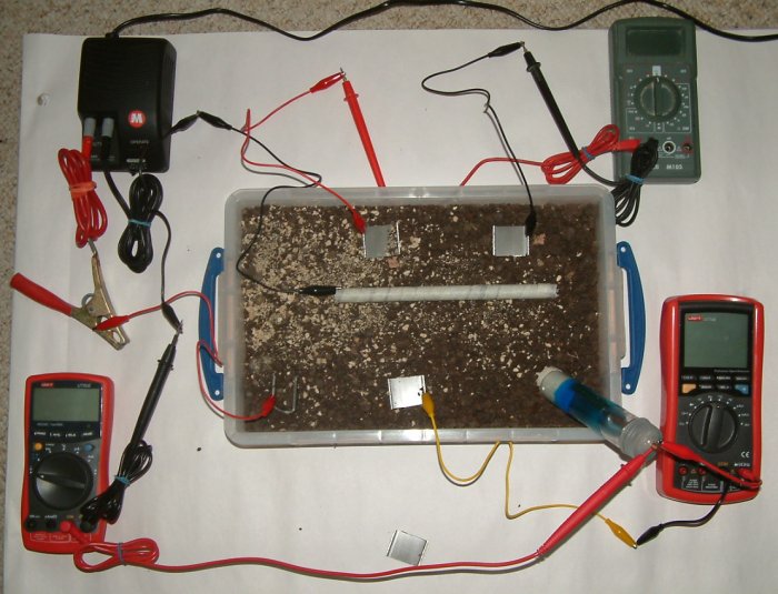
You can see the power supply in the top left hand corner of the picture that is pumping charges through the red lead (with the massive croc clip) through the small red lead to a piece of steel buried in the earth in the bottom left corner of the plastic tray.

The short length of steel pipe is coated with a material that is conductive when wet. This is set in the soil and connected to the negative terminal of the DC power supply.

The negative power supply connection is split into two, one of which is connected to the pipe wrapped in white tape in the centre of the tray and the other connected to the black terminal of the multimeter in the bottom left corner of the picture.
The red terminal of this multimeter is connected to the Cu/CuSO4 electrode in the bottom right hand corner of the tray rendering a 'pipe-to-soil' voltage on that meter.



The grey multimeter at the top right of the picture is connected between two identical pieces of steel that serve as ground contact electrodes at the top of the tray. The measurement on this meter will reflect the potential of the earth at the points of contact and this will show the potential gradient resulting from the currents in the tray.

The multimeter in the bottom right of the picture is connected to a piece of steel placed in the botton centre of the tray and the Cu/CuSO4 electrode. It will display the voltage resulting from the difference in potential of the earth in the bottom centre of the tray and the potential of the Cu/CuSO4 electrode. The Cu/CuSO4 potential is used as a reference between the pipe and the soil potentials in this case only.



It should be noted that the readings on the grey multimeter are not related to the potentials measured on the other two multimeters as there is no common reference. The purpose of these measurements is to observe the potential gradient within the tray as it is influenced by the corrosion reactions of metal to the electrolyte and the charges impressed into the tray.



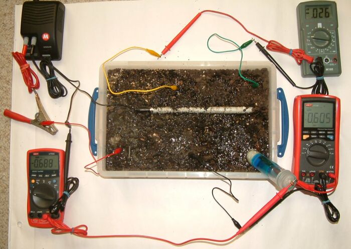
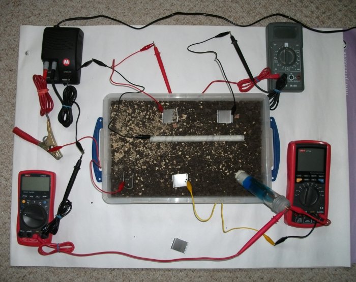
The picture above was taken before the power supply was energised and the measurements on the meters might be regarded as 'native' conditions by some corrosion specialists. However, they only serve as a starting point in our observations of the changes in earth potentials in relation to the earth potential at the point of contact with the Cu/CuSO4 electrode.



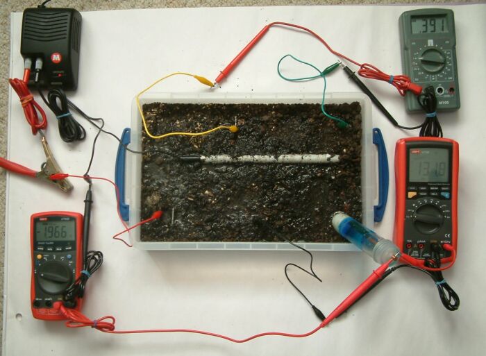
In the picture above we can see that the power supply has been energised and the 'pipe-to-soil potential' shown on the bottom left multimeter is -1.966 volts. the voltage between the steel electrode at the centre bottom ogf the tray and the Cu/CuSO4 electrode is 1.318 volts and it should be noted that the test leads are connected in the opposite way to those on the bottom left mulitmeter.



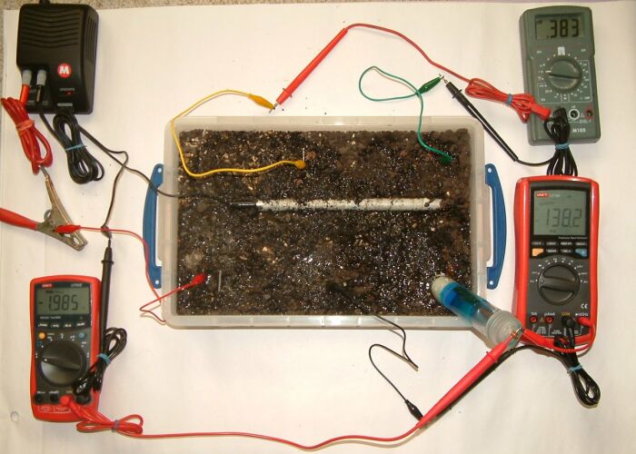
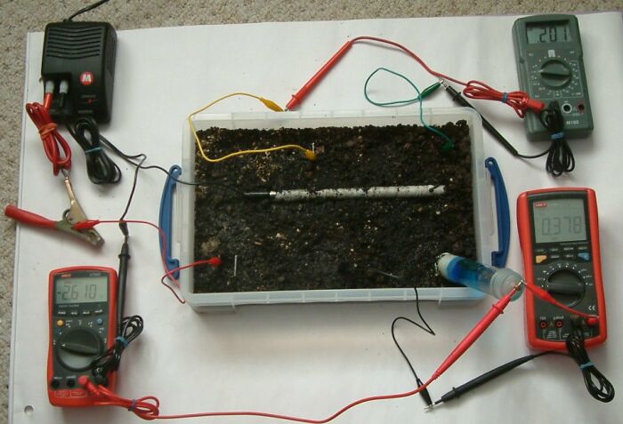
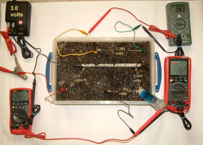
In this picture it can be seen that the readings have changed and the pipe-to-soil potential is shown as -1.985 volts, the independant steel coupn at the bottom of the tray is 1.382 volts in relation to the Cu/CuSO4 electrode and the voltage between the two independent electrodes at the top of the tray is shown on the grey multimeter as 0.383 volts.



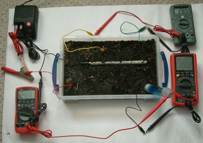
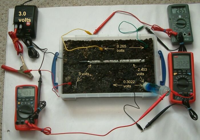
in the picture above you can see that the pipe to soil is now -2.403 volts the centre bottome electrode is 302.2mv and the voltage between the top two electrode is 0.265 volts.



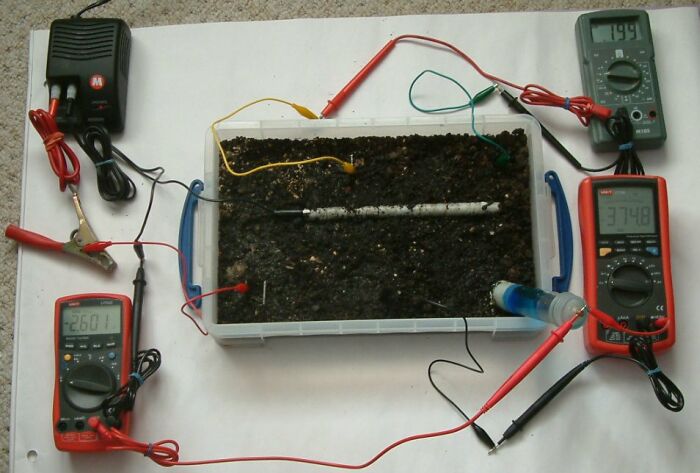
In this picture the pipe-to-soil is -2.601 volts, the centre bottom electrode is 374.8mv and the voltage between the top two electrode is 0.199v.



In this picture the pipe to soil is -2.610 volts, the middle bottom electrode is 0.378mv and the voltage between the top two electrodes is 0.201 volts



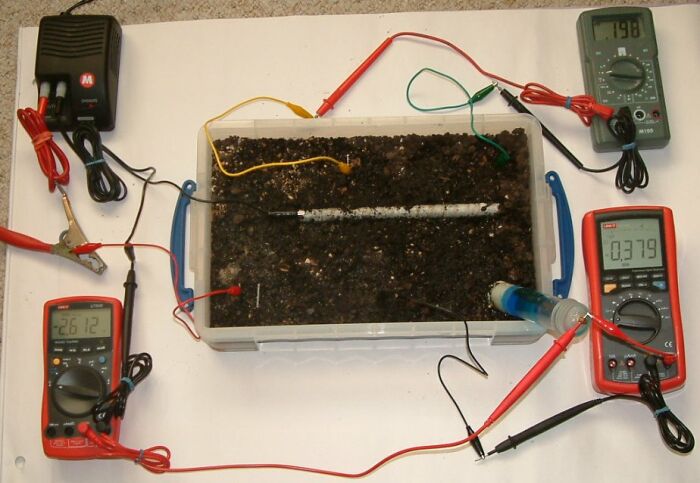
In this picture the pipe to soil potential is -2.612 volts, the centre bottom electrode is 0.379 volts and the voltage between the top two electrodes is 0.198v.



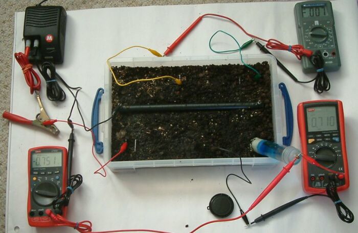
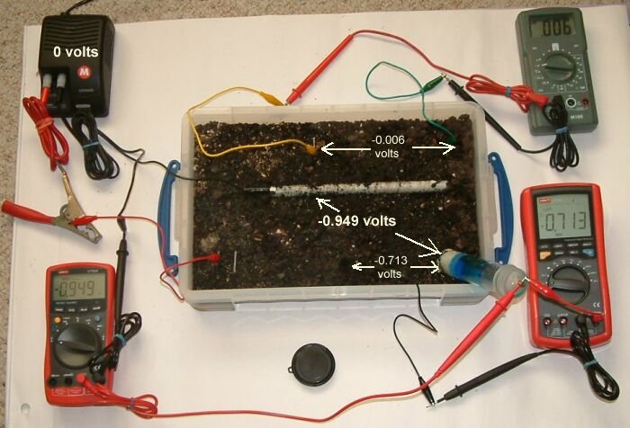
In this picture the pipe to soil potential is shown as -0.949 volts and the power supply is switched off. The centre bottom electrode is 0.713 volts and the voltage between the top two electrodes is 0.006v



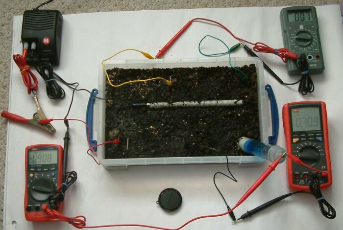
In this picture the pipe to soil potential is -0.908 volts, the centre electrode is 0.709 volts and the voltage between the top two electrodes is 0.007v.



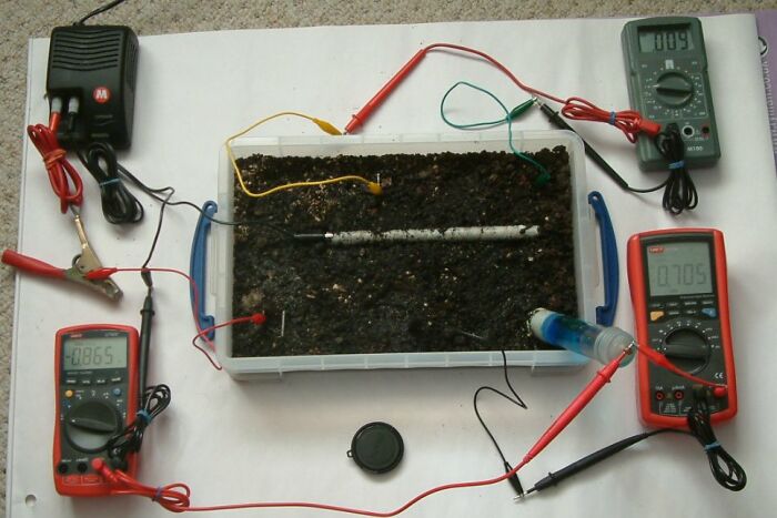
In this picture the pipe to soil potential is =0.865 volts, the centre bottom electrode is 0.705 volts and the voltage between the top two electrodes is 0.009v.



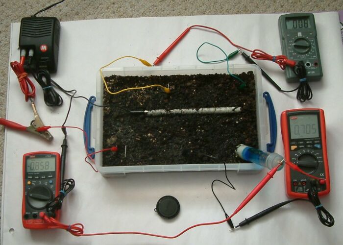
In this picture the pipe to soil potential is -0.858 volts, the centre electrode is 0.705 volts and the voltage between the two top electrodes is 0.008v.

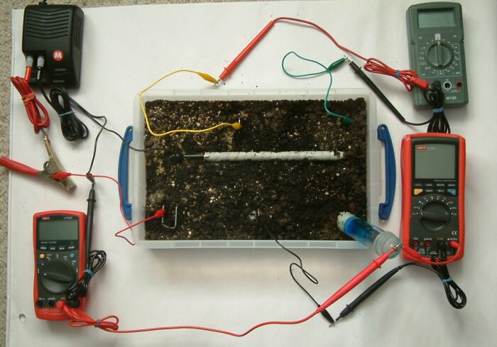
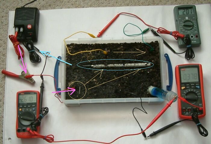
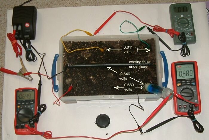
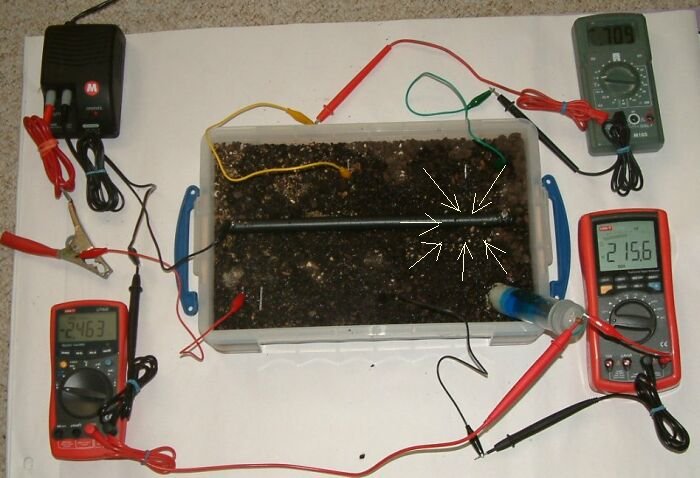
The steel pipe is changed to one coated with insulation tape.



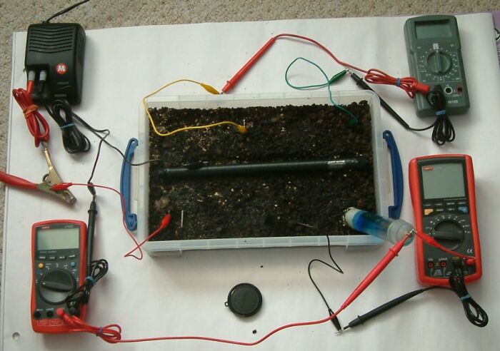
This has a coating fault on the underside that will be in contact with the earth.



This pipe is fitted with electrical contacts of mild steel on top for convenience of experimentation. There are no bi-metalic couplings present on this test piece.



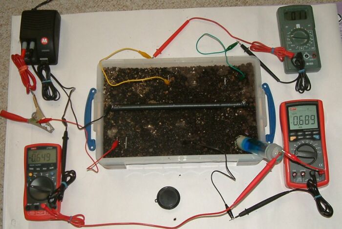
The meters are turned on but not the DC power supply, so the readings are 'unprotected' but the steel ground contact electrodes have been electrically altered during the previous experiments, so the equilibrium of this model cannot be regarded as 'natural'.



It can be seen that there is a voltage of -0.649 between the pipe metal and the Cu/CuSO4 electrode. There is a voltage of 0.689 between the steel electrode placed at the centre bottom of the tray and the Cu/CuSO4 electrode. You will note that the connections between the probes and the meters have been deliberately reversed to demonstrate that the multimeter is incapable of reasoning and that it simply asigns a zero according to one pole of the meter. The - sign is asigned by the meter as it is set up to make a measurement.



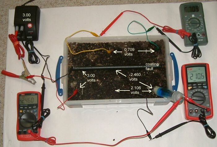
The power supply is energised (as seen by the tiny red dot) and the charges are defusing through the least line of resistance to complete the circuit.



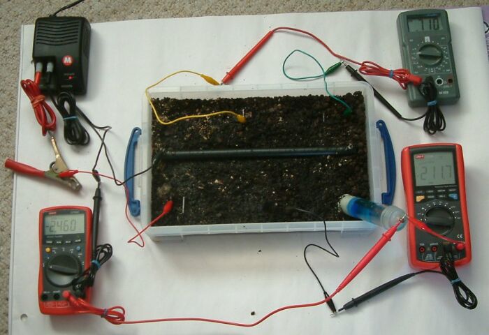
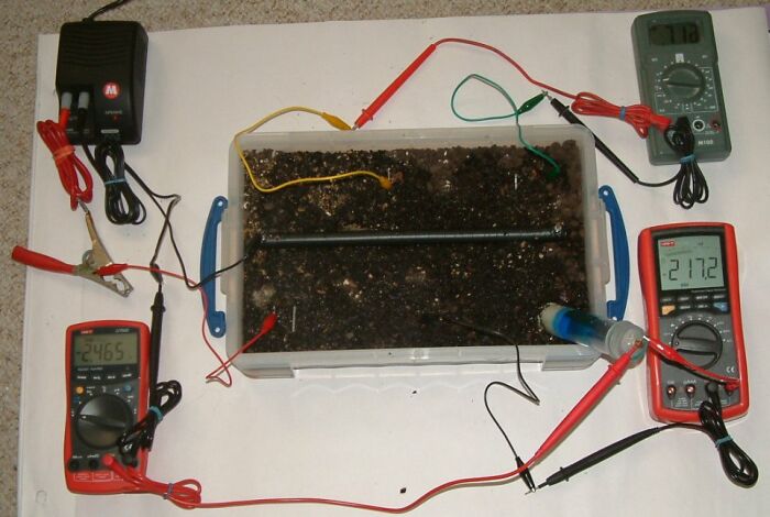
You can see that the voltage between the Cu/CuSO4 electrode in the bottom right hand corner of the tray and the exposed steel of the pipe in the 12 oclock positon above it in the picture is -2.460v. The voltage between the steel earth contact electrode in the centre bottom of the tray and the Cu/CuSO4 electrode is 2.117v and the voltage between the top two steel electrodes is 1.10v, shown on the grey multimeter.



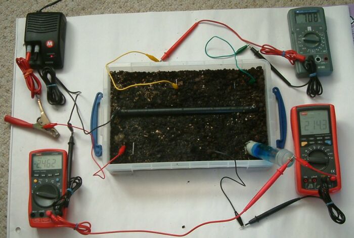
In this picture you can see that the voltages are changing with time as the corrosion equilibrium is altered by the cathodic protection current.



This next picture was taken using flash that masked the tiny red dot on the power supply, that was still energised at this time.



This second picture taken using flash, shows that the voltages on all meters are increasing slightly which indicates that the potential of the earth is changing. Each voltage is relative to another earth voltage and none are related to the actual interface potential required by science, that is measured at the ANODIC interface.



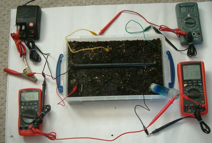
It can be seen that the power supply is still energised and that the pipe-to-soil voltage on the bottom left multimeter is at 2.466v and the bottom right multimeter is 2.178v. This begs the question 'wha are we measuring' as the steel earth electrode in the centre bottom of the tray is not connected to the cathodic protection system in any way?



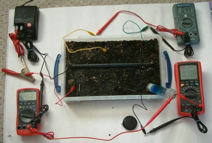
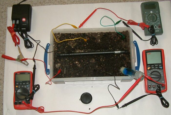
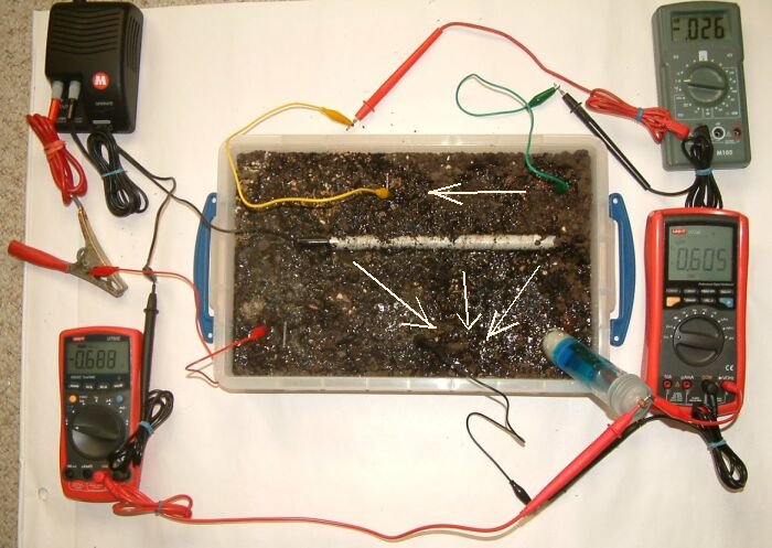
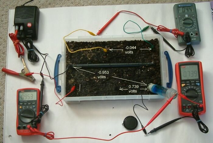
In this next picture the power supply is off and the potential gradient in the earth is reducing. The significant measurment is seen in the grey multimeter that is now at -0.44v. The earth between the two steel electrodes has reversed it's potential polarity with repect to this meter.
The 'pipe-to-soil' potential of the pipe is shown as -0.953v on the left hand bottom multimeter and the voltage between the steel earth electrode in the bottom centre of the tray and the CU/CuSO4 electrode is shown on the left hand bottom multimenter as 0.739v.



A few seconds later you can see that the values are reducing as the system recovers equilibrium in the abscence of any impressed electrical charges.



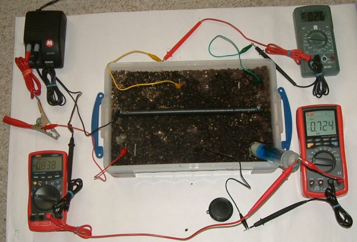
A few seconds later and the system continues to change in what has become known as depolarisation.



These experiments show the electrical status of the earth potentials in respect to the passage of DC electrical charges that are impressed y w power supply or by galvanic action in the case of sacrificial anode systems of cathodic protection.

Any doubts about that can be replicated in these demonstrations usin sacrificial anodes or dry cell batteries.

By perceiving electrical potential as pressure and understanding that a digital voltmeter sets its own zero for each measurement, we also realise that the polarity sign is a function of the way we connect the meter to the subject to be measured.



This assumption can be tested by playing about with the connections and getting the 'feel' of the behaviour of electrical charges in the electrolyte.



We can extend this 'visualisation' to each experiment and build the ability to understand the nature of cathodic protection.



By seeing the meter display you know that the electrical pressure at the steel connected to the positive side of the power supply has charged up the earth to the value of 1.966 volts with respect to the potential of the Cu/CuSO4 electrode.
The charges disperse to all parts of the earth in the tray but the pipe is drained of charges so that it depletes the potential of the earth around it.



We are relating the Cu/CuSO4 electrode to the bottom two multimeters but have connected them in different ways to illustrate that we can only measure a potential difference which we call a voltage.



We must look at the polarity of each measurement and the common reference of two measurements to work out the relationship between any two potentials in a system.



It can be seen that the two electrodes at the top of the tray have no common zero and we can only know the polarity and voltage between the earth contact points.



This does tell us the direction of low of the charges between the top wlectrodes.



We have switched of the power supply but none of the multimeters has reversed their polarity indicators so the current is still passing int the same direction.



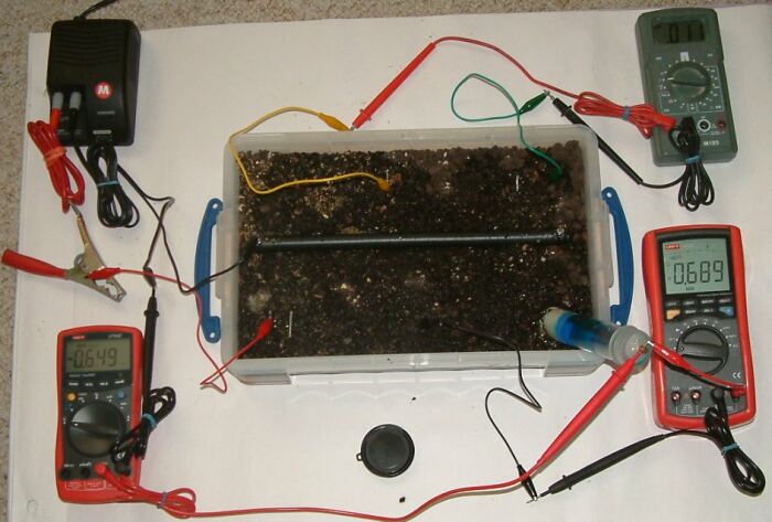
The pipe has been replaced with an insulated pipe with a coating fault under the farthest end from the power supply that has not yet been switched on. The charges shown on the meters must result from different reactions at each steel interface with the earth.



The power supply has been energised to 3 volts and that is the potential difference between the steel anode and the whole of the length of pipe.
The steel at the coating fault is the only place that the charges can complete their circuitand in doing so they pass through shells of resistance that allow the potential profile of the earth to be measured.



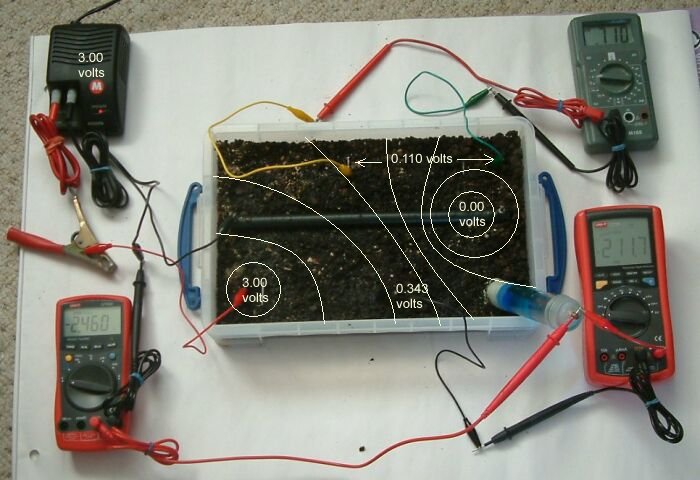
We can plot the 'isopotential' contours of the tray in the same way that we plot groundbed profiles and discover DCVG coating faults.



Charges difuse something like radiation but also like expansion to fill every available partical until they meet a greater resistance. It is scientific nonsense to think that charges follow straight lines as photons do.



Charges 'seek' a return path to zero follwing the rules of physics codifed by Kirckoff in that they pass in inverse proportion to the resistances they encounter. It is for this reason that the total resistance increases as the charges encounter less and less resistances in parallel, forming the shells of resistance described in scientific papers by Dr's Prinz, Baekmann, Baaltz, Schwenke and many others.



In this picture the power supply has been switched off and it can be seen that the potential profile of the earth in the tray has changed the readings on the meters. Remember that the bottom two meters have their leads connected in different polarity so we can ignor the polarity negative sign.
The pipeline coating reduces the surface area of the pipe and alters the location of access for the charges. The charges remaining in the top right hand corner of the tray are greater than those remaining in the centre of the top of the tray reversing the polarity of the grey meter. The readings on this meter are not refered to a common potential on either of the meters below.



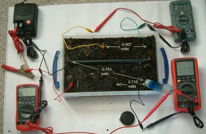
It is clear that the coating changed the behaviour of the charges impressed into this cathodic protection system by concentrating the CP current on the exposed area and not allowing access to the pipeline metal in the immediate area of influence of the anode.



It is clear that the best coating from a cathodic protection point of view is that which has the best electrical insulating properties.

Any areas that allow cathodic protection current to enter the structure or pipeline metal reduce the spread of protective charges.

Cathodic protection not only reduces the energy in the pipeline to below it's corrosion potential but increases the potential of the electrolyte at the anodic interface of a corrosion cell.

It is when this electrolytic potential is greater than the EMF of the corrosion reaction that cathodic protection stops metal going into solution.

We cannot measure electrons and do not measure pH values extensively in field work but we gather voltages and it is from these that we are able to adjust our cathodic protection systems to prevent corrosion at coating faults,

Any suggestion that we can use conductive coating with cathodic protection is likely to be based on commercial advantage as there is no scientific basis.